zero padding
Смотреть что такое «zero padding» в других словарях:
Padding — (von engl. to pad für auffüllen) ist ein Fachbegriff der Informatik für Fülldaten, mit denen ein vorhandener Datenbestand vergrößert wird. Die Füllbytes werden auch Pad Bytes genannt. Die für Prüfsummen verwendeten Daten zählen hierbei nicht zum… … Deutsch Wikipedia
F-Zero X — Infobox VG| title = F Zero X developer = Nintendo EAD publisher = Nintendo designer = Shigeru Miyamoto (producer)cite web | url=http://www.gamespot.com/n64/driving/fzero10/tech info.html | accessdate=2008 08 30 | publisher= GameSpot | title=F… … Wikipedia
Base64 — Numeral systems by culture Hindu Arabic numerals Western Arabic (Hindu numerals) Eastern Arabic Indian family Tamil Burmese Khmer Lao Mongolian Thai East Asian numerals Chinese Japanese Suzhou Korean Vietnamese … Wikipedia
Bluestein’s FFT algorithm — (1968), commonly called the chirp z transform algorithm (1969), is a fast Fourier transform (FFT) algorithm that computes the discrete Fourier transform (DFT) of arbitrary sizes (including prime sizes) by re expressing the DFT as a convolution.… … Wikipedia
Rader’s FFT algorithm — Rader s algorithm (1968) is a fast Fourier transform (FFT) algorithm that computes the discrete Fourier transform (DFT) of prime sizes by re expressing the DFT as a cyclic convolution. (The other algorithm for FFTs of prime sizes, Bluestein s… … Wikipedia
Ciphertext stealing — In cryptography, ciphertext stealing (CTS) is a general method of using a block cipher mode of operation that allows for processing of messages that are not evenly divisible into blocks without resulting in any expansion of the ciphertext, at the … Wikipedia
Luhn algorithm — The Luhn algorithm or Luhn formula, also known as the modulus 10 or mod 10 algorithm, is a simple checksum formula used to validate a variety of identification numbers, such as credit card numbers, IMEI numbers, National Provider Identifier… … Wikipedia
The Cat Came Back — Infobox Standard title= The Cat Came Back comment= image size= caption=Cover, sheet music, 1893 writer=Harry S. Miller composer= lyricist= published= 1893 written= language=English form= original artist= recorded by= performed by= The Cat Came… … Wikipedia
Schnelle Faltung — Die Schnelle Faltung ist ein Algorithmus zur Berechnung der diskreten, aperiodischen Faltungsoperation mit Hilfe der schnellen Fourier Transformation (FFT). Dabei wird die rechenintensive aperiodische Faltungsoperation im Zeitbereich durch eine… … Deutsch Wikipedia
zero padding
дополнение нулями
Дополнение кадра до требуемого фиксированного размера путем заполнения свободных позиций последовательностью, состоящей из одних нулей.
[Л.М. Невдяев. Телекоммуникационные технологии. Англо-русский толковый словарь-справочник. Под редакцией Ю.М. Горностаева. Москва, 2002]
Тематики
Смотреть что такое «zero padding» в других словарях:
Padding — (von engl. to pad für auffüllen) ist ein Fachbegriff der Informatik für Fülldaten, mit denen ein vorhandener Datenbestand vergrößert wird. Die Füllbytes werden auch Pad Bytes genannt. Die für Prüfsummen verwendeten Daten zählen hierbei nicht zum… … Deutsch Wikipedia
F-Zero X — Infobox VG| title = F Zero X developer = Nintendo EAD publisher = Nintendo designer = Shigeru Miyamoto (producer)cite web | url=http://www.gamespot.com/n64/driving/fzero10/tech info.html | accessdate=2008 08 30 | publisher= GameSpot | title=F… … Wikipedia
Base64 — Numeral systems by culture Hindu Arabic numerals Western Arabic (Hindu numerals) Eastern Arabic Indian family Tamil Burmese Khmer Lao Mongolian Thai East Asian numerals Chinese Japanese Suzhou Korean Vietnamese … Wikipedia
Bluestein’s FFT algorithm — (1968), commonly called the chirp z transform algorithm (1969), is a fast Fourier transform (FFT) algorithm that computes the discrete Fourier transform (DFT) of arbitrary sizes (including prime sizes) by re expressing the DFT as a convolution.… … Wikipedia
Rader’s FFT algorithm — Rader s algorithm (1968) is a fast Fourier transform (FFT) algorithm that computes the discrete Fourier transform (DFT) of prime sizes by re expressing the DFT as a cyclic convolution. (The other algorithm for FFTs of prime sizes, Bluestein s… … Wikipedia
Ciphertext stealing — In cryptography, ciphertext stealing (CTS) is a general method of using a block cipher mode of operation that allows for processing of messages that are not evenly divisible into blocks without resulting in any expansion of the ciphertext, at the … Wikipedia
Luhn algorithm — The Luhn algorithm or Luhn formula, also known as the modulus 10 or mod 10 algorithm, is a simple checksum formula used to validate a variety of identification numbers, such as credit card numbers, IMEI numbers, National Provider Identifier… … Wikipedia
The Cat Came Back — Infobox Standard title= The Cat Came Back comment= image size= caption=Cover, sheet music, 1893 writer=Harry S. Miller composer= lyricist= published= 1893 written= language=English form= original artist= recorded by= performed by= The Cat Came… … Wikipedia
Schnelle Faltung — Die Schnelle Faltung ist ein Algorithmus zur Berechnung der diskreten, aperiodischen Faltungsoperation mit Hilfe der schnellen Fourier Transformation (FFT). Dabei wird die rechenintensive aperiodische Faltungsoperation im Zeitbereich durch eine… … Deutsch Wikipedia
FFT Zero Padding
The Fast Fourier Transform (FFT) is one of the most used tools in electrical engineering analysis, but certain aspects of the transform are not widely understood–even by engineers who think they understand the FFT. Some of the most commonly misunderstood concepts are zero-padding, frequency resolution, and how to choose the right Fourier transform size.
This article will explore zero-padding the Fourier transform–how to do it correctly and what is actually happening. The exploration will cover of the following topics:
Zero Padding
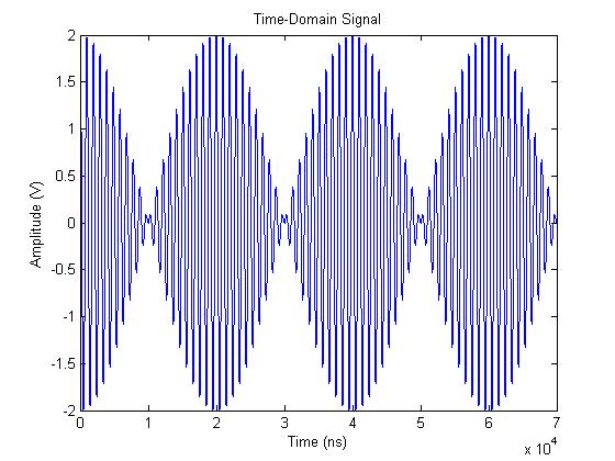
Zero padding is a simple concept; it simply refers to adding zeros to end of a time-domain signal to increase its length. The example 1 MHz and 1.05 MHz real-valued sinusoid waveforms we will be using throughout this article is shown in the following plot:
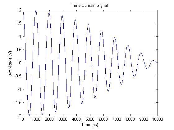
The time-domain length of this waveform is 1000 samples. At the sampling rate of 100 MHz, that is a time-length of 10 us. If we zero pad the waveform with an additional 1000 samples (or 10 us of data), the resulting waveform is produced:
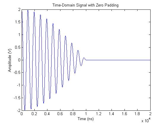
There are a few reasons why you might want to zero pad time-domain data. The most common reason is to make a waveform have a power-of-two number of samples. When the time-domain length of a waveform is a power of two, radix-2 FFT algorithms, which are extremely efficient, can be used to speed up processing time. FFT algorithms made for FPGAs also typically only work on lengths of power two.
While it’s often necessary to stick to powers of two in your time-domain waveform length, it’s important to keep in mind how doing that affects the resolution of your frequency-domain output.
FFT Frequency Resolution
There are two aspects of FFT resolution. I’ll call the first one “waveform frequency resolution” and the second one “FFT resolution”. These are not technical names, but I find them helpful for the sake of this discussion. The two can often be confused because when the signal is not zero padded, the two resolutions are equivalent.
The “waveform frequency resolution” is the minimum spacing between two frequencies that can be resolved. The “FFT resolution” is the number of points in the spectrum, which is directly proportional to the number points used in the FFT.
It is possible to have extremely fine FFT resolution, yet not be able to resolve two coarsely separated frequencies.
It is also possible to have fine waveform frequency resolution, but have the peak energy of the sinusoid spread throughout the entire spectrum (this is called FFT spectral leakage).
The waveform frequency resolution is defined by the following equation:

where T is the time length of the signal with data. It’s important to note here that you should not include any zero padding in this time! Only consider the actual data samples.
It’s important to make the connection here that the discrete time Fourier transform (DTFT) or FFT operates on the data as if it were an infinite sequence with zeros on either side of the waveform. This is why the FFT has the distinctive sinc function shape at each frequency bin.
You should recognize the waveform resolution equation 1/T is the same as the space between nulls of a sinc function.
The FFT resolution is defined by the following equation:
Frequency Domain Resolution Concept Exploration
Considering our example waveform with 1 V-peak sinusoids at 1 MHz and 1.05 MHz, let’s start exploring these concepts.
Let’s start off by thinking about what we should expect to see in a power spectrum. Since both sinusoids have 1 Vpeak amplitudes, we should expect to see spikes in the frequency domain with 10 dBm amplitude at both 1 MHz and 1.05 MHz.
The original time-domain signal shown in the first plot with a length of 1000 samples (10 us). A 1000-point FFT used on the time-domain signal is shown in the next figure:

Two distinct peaks are not shown, and the single wide peak has an amplitude of about 11.4 dBm. Clearly these results don’t give an accurate picture of the spectrum. There is not enough resolution in the frequency domain to see both peaks.
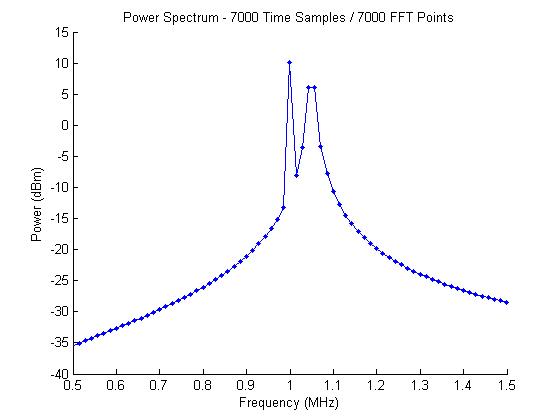
Let’s try to resolve the two peaks in the frequency domain by using a larger FFT, thus adding more points to the spectrum along the frequency axis. Let’s use a 7000-point FFT. This is done by zero padding the time-domain signal with 6000 zeros (60 us). The zero-padded time-domain signal is shown here:
The resulting frequency-domain data, shown as a power spectrum, is shown here:

Although we’ve added many more frequency points, we still cannot resolve the two sinuoids; we are also still not getting the expected power.
Taking a closer look at what this plot is telling us, we see that all we have done by adding more FFT points is to more clearly define the underlying sinc function arising from the waveform frequency resolution equation. You can see that the sinc nulls are spaced at about 0.1 MHz.
Because our two sinusoids are spaced only 0.05 MHz apart, no matter how many FFT points (zero padding) we use, we will never be able to resolve the two sinusoids.
Let’s look at what the resolution equations are telling us. Although the FFT resolution is about 14 kHz (more than enough resoution), the waveform frequency resolution is only 100 kHz. The spacing between signals is 50 kHz, so we are being limited by the waveform frequency resolution.
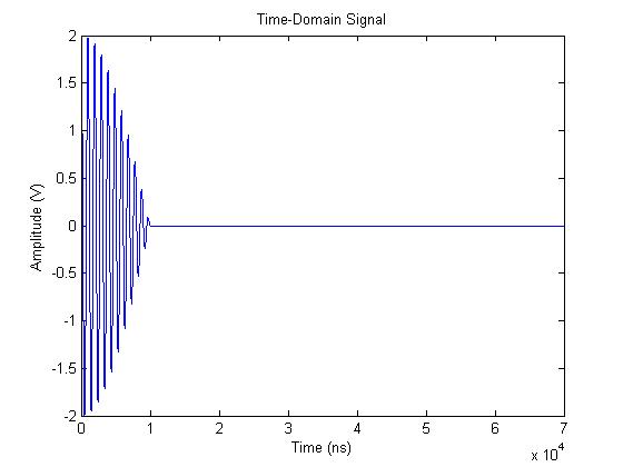
To resolve the spectrum properly, we need to increase the amount of time-domain data we are using. Instead of zero padding the signal out to 70 us (7000 points), let’s capture 7000 points of the waveform. The time-domain and domain results are shown here, respectively.
The resulting frequency-domain data, shown as a power spectrum, is shown here:
With the expanded time-domain data, the waveform frequency resolution is now about 14 kHz as well. As seen in the power spectrum plot, the two sinusoids are not seen. The 1 MHz signal is clearly represented and is at the correct power level of 10 dBm, but the 1.05 MHz signal is wider and not showing the expected power level of 10 dBm. What gives?
What is happening with the 1.05 MHz signal is that we don’t have an FFT point at 1.05 MHz, so the energy is split between multiple FFT bins.
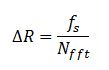
The spacing between FFT points follows the equation:
where nfft is the number of FFT points and fs is the sampling frequency.
In our example, we’re using a sampling frequency of 100 MHz and a 7000-point FFT. This gives us a spacing between points of 14.28 kHz. The frequency of 1 MHz is a multiple of the spacing, but 1.05 MHz is not. The closest frequencies to 1.05 MHz are 1.043 MHz 1.057 MHz, so the energy is split between the two FFT bins.
To solve this issue, we can choose the FFT size so that both frequencies are single points along the frequency axis. Since we don’t need finer waveform frequency resolution, it’s okay to just zero pad the time-domain data to adjust the FFT point spacing.
Adding an additional 1000 zeros (10 us) to the time-domain signal gives us a spacing of 12.5 kHz, and both 1 MHz and 1.05 MHz are integer multiples of the spacing. The resulting spectrum is shown in the following figure.
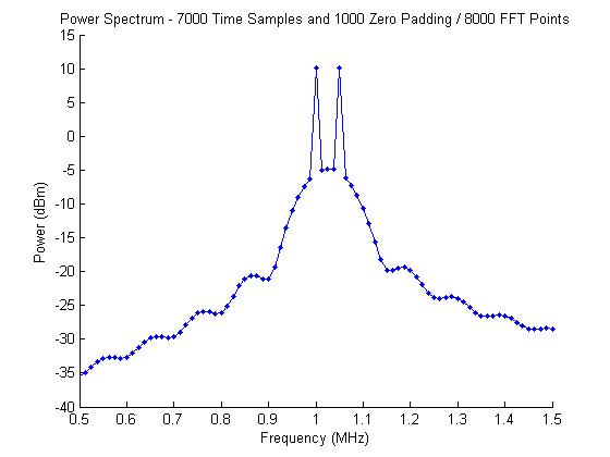
Now both frequencies are resolved and at the expected power of 10 dBm.
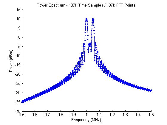
For the sake of overkill, you can always add more points to your FFT through zero padding (ensuring that you have the correct waveform resolution) to see the shape of the FFT bins as well. This is shown in the following figure:
Choosing the Right FFT Size
Three considerations should factor into your choice of FFT size, zero padding, and time-domain data length.
1) The waveform frequency resolution should be smaller than the minimum spacing between frequencies of interest.
2) The FFT resolution should at least support the same resolution as your waveform frequency resolution. Additionally, some highly-efficient implementations of the FFT require that the number of FFT points be a power of two.
3) You should ensure that there are enough points in the FFT, or the FFT has the correct spacing set, so that your frequencies of interest are not split between multiple FFT points.
One final thought on zero padding the FFT:
If you apply a windowing function to your waveform, the windowing function needs to be applied before zero padding the data. This ensures that your real waveform data starts and ends at zero, which is the point of most windowing functions.
Thanks for reading!
We want to hear from you! Do you have a comment, question, or suggestion? Twitter us @bitweenie or me @shilbertbw, or leave a comment right here!
Why should I zero-pad a signal before taking the Fourier transform?
In an answer to a previous question, it was stated that one should
zero-pad the input signals (add zeros to the end so that at least half of the wave is «blank»)
What’s the reason for this?
6 Answers 6
Zero padding allows one to use a longer FFT, which will produce a longer FFT result vector.
A longer FFT result has more frequency bins that are more closely spaced in frequency. But they will be essentially providing the same result as a high quality Sinc interpolation of a shorter non-zero-padded FFT of the original data.
This might result in a smoother looking spectrum when plotted without further interpolation.
Although this interpolation won’t help with resolving or the resolution of and/or between adjacent or nearby frequencies, it might make it easier to visually resolve the peak of a single isolated frequency that does not have any significant adjacent signals or noise in the spectrum. Statistically, the higher density of FFT result bins will probably make it more likely that the peak magnitude bin is closer to the frequency of a random isolated input frequency sinusoid, and without further interpolation (parabolic, et.al.).
But, essentially, zero padding before a DFT/FFT is a computationally efficient method of interpolating a large number of points.
Zero-padding for cross-correlation, auto-correlation, or convolution filtering is used to not mix convolution results (due to circular convolution). The full result of a linear convolution is longer than either of the two input vectors. If you don’t provide a place to put the end of this longer convolution result, FFT fast convolution will just mix it in with and cruft up your desired result. Zero-padding provides a bunch zeros into which to mix the longer result. And it’s far far easier to un-mix something that has only been mixed/summed with a vector of zeros.

There are a few things to consider before you decide to zero pad your time-domain signal. You may not need to zero pad the signal at all!
1) Lengthen the time-domain data (not zero padding) to get better resolution in the frequency domain.
2) Increase the number of FFT points beyond your time-domain signal length (zero padding) if you would like to see better definition of the FFT bins, though it doesn’t buy you any more true resolution. You can also pad to get to a power of 2 number of FFT points.
There are some nice figures illustrating these points at http://www.bitweenie.com/listings/fft-zero-padding/
One last thing to mention: If you zero pad the signal in the time domain and you want to use a windowing function, make sure you window the signal before you zero pad. If you apply the window function after zero padding, you won’t accomplish what the window is supposed to accomplish. More specifically, you’ll still have a sharp transition from the signal to zero instead of a smooth transition to zero.

In general zero-padding prior to DFT is equivalent to interpolation, or sampling more often, in the transformed domain.
Here is a quick visualization of how the opposite works. If you sample a bandlimited signal in time at higher rate, you get a more ‘squashed’ spectrum, i.e. a spectrum with more zeros at both ends. In other words, you can obtain more samples in time by simply zero-padding in frequency after DFT’ing, and then IDFT’ing the zero-padded result.
The same effect holds in reverse when zero-padding occurs in time. This is all because the perfect signal reconstruction is possible as long as a signal is bandlimited and sampled at least at the Nyquist rate.
The term ‘resolution’ depends on how you define it. For me, it means how well the two adjacent points of observation in time or frequency can be reliably (statistically) discriminated. In this case the resolution actually depends on the DFT size due to spectral leakage. That is, smaller the window size, more blurry or smeared the transformed signal, and vice versa. It is different from how often you sample, or what I term ‘definition’. For example, you can have a very blurry image sampled at high rate (high definition), yet you still cannot obtain more information than sampling at lower rate. So in summary, zero-padding does not improve resolution at all since you do not gain any more information than before.

If one has any interest in the spectrum of the windowing function used to isolate the time-domain sample, then zero-padding WILL increase the frequency resolution of the windowing function.
There can be different reasons for this depending on any processes carried out before and after the Fourier transform. The most common reason is to achieve greater frequency resolution in any resulting transform. That is to say that, the larger the number of samples used in your transform, the narrower the binwidth in the resulting power spectrum. Remember: binwidth = sample_frequency/transform_size (often called window size). You can imagine from this, that as you increase your transform size, binwidth reduces (=better frequency resolution). Zero padding is a way of increasing the transform size without introducing new information to the signal.
So why not just take a bigger transform without zero padding? Would that not achieve the same effect? Good question. In many cases you may want to analyze a stream of time domain data, for which you may be using a short time Fourier transform (stft). This involves taking a transform every N samples according to the time resolution you need in order to characterize changes in the frequency spectrum. Here in lies the problem. Too big a window and you will lose time resolution, too small a window and you will lose frequency resolution. The solution then is to take small time domain windows giving you good time resolution and then zero pad them to give you good frequency resolution. Hope this is useful for you
Machine Learning & Deep Learning Fundamentals
Zero Padding in Convolutional Neural Networks explained
video
Zero Padding in Convolutional Neural Networks
What’s going on everyone? In this post, we’re going to discuss zero padding as it pertains to convolutional neural networks. What the heck is this mysterious concept? We’re about to find out, so let’s get to it.

We’re going to start out by explaining the motivation for zero padding, and then we’ll get into the details about what zero padding actually is. We’ll then talk about the types of issues we may run into if we don’t use zero padding, and then we’ll see how we can implement zero padding in code using Keras.
We’re going to be building on some of the ideas that we discussed in our post on convolutional neural networks, so if you haven’t seen that yet, go ahead and check it out, and then come back to to this one once you’ve finished up there.
Convolutions reduce channel dimensions
We’ve seen in our post on CNNs that each convolutional layer has some number of filters that we define, and we also define the dimension of these filters as well. We also showed how these filters convolve image input.
When a filter convolves a given input channel, it gives us an output channel. This output channel is a matrix of pixels with the values that were computed during the convolutions that occurred on the input channel.
When this happens, the dimensions of our image are reduced.
Let’s check this out using the same image of a seven that we used in our previous post on CNNs. Recall, we have a 28 x 28 matrix of the pixel values from an image of a 7 from the MNIST data set. We’ll use a 3 x 3 filter. This gives us the following the items:
A 28 x 28 single input channel (grayscale image):
| 0.0 | 0.0 | 0.0 | 0.0 | 0.0 | 0.0 | 0.0 | 0.0 | 0.0 | 0.0 | 0.0 | 0.0 | 0.0 | 0.0 | 0.0 | 0.0 | 0.0 | 0.0 | 0.0 | 0.0 | 0.0 | 0.0 | 0.0 | 0.0 | 0.0 | 0.0 | 0.0 | 0.0 |
| 0.0 | 0.0 | 0.0 | 0.0 | 0.0 | 0.0 | 0.0 | 0.0 | 0.0 | 0.0 | 0.0 | 0.0 | 0.0 | 0.0 | 0.0 | 0.0 | 0.0 | 0.0 | 0.0 | 0.0 | 0.0 | 0.0 | 0.0 | 0.0 | 0.0 | 0.0 | 0.0 | 0.0 |
| 0.0 | 0.0 | 0.0 | 0.0 | 0.0 | 0.0 | 0.0 | 0.0 | 0.0 | 0.0 | 0.0 | 0.0 | 0.0 | 0.0 | 0.0 | 0.0 | 0.0 | 0.0 | 0.0 | 0.0 | 0.0 | 0.0 | 0.0 | 0.0 | 0.0 | 0.0 | 0.0 | 0.0 |
| 0.0 | 0.0 | 0.0 | 0.0 | 0.0 | 0.0 | 0.0 | 0.0 | 0.0 | 0.0 | 0.0 | 0.0 | 0.0 | 0.0 | 0.0 | 0.0 | 0.0 | 0.0 | 0.0 | 0.0 | 0.0 | 0.0 | 0.0 | 0.0 | 0.0 | 0.0 | 0.0 | 0.0 |
| 0.0 | 0.0 | 0.0 | 0.0 | 0.0 | 0.0 | 0.0 | 0.0 | 0.0 | 0.0 | 0.0 | 0.0 | 0.0 | 0.0 | 0.0 | 0.0 | 0.0 | 0.0 | 0.0 | 0.0 | 0.0 | 0.0 | 0.0 | 0.0 | 0.0 | 0.0 | 0.0 | 0.0 |
| 0.0 | 0.0 | 0.0 | 0.0 | 0.0 | 0.0 | 0.0 | 0.0 | 0.0 | 0.0 | 0.0 | 0.0 | 0.0 | 0.0 | 0.0 | 0.0 | 0.0 | 0.0 | 0.0 | 0.0 | 0.0 | 0.0 | 0.0 | 0.0 | 0.0 | 0.0 | 0.0 | 0.0 |
| 0.0 | 0.0 | 0.0 | 0.0 | 0.0 | 0.0 | 0.0 | 0.0 | 0.0 | 0.0 | 0.0 | 0.0 | 0.0 | 0.0 | 0.0 | 0.0 | 0.0 | 0.0 | 0.0 | 0.0 | 0.0 | 0.0 | 0.0 | 0.0 | 0.0 | 0.0 | 0.0 | 0.0 |
| 0.0 | 0.0 | 0.0 | 0.0 | 0.0 | 0.0 | 0.0 | 0.0 | 0.0 | 0.0 | 0.0 | 0.4 | 0.4 | 0.3 | 0.5 | 0.2 | 0.0 | 0.0 | 0.0 | 0.0 | 0.0 | 0.0 | 0.0 | 0.0 | 0.0 | 0.0 | 0.0 | 0.0 |
| 0.0 | 0.0 | 0.0 | 0.4 | 0.5 | 0.9 | 0.9 | 0.9 | 0.9 | 0.9 | 0.9 | 1.0 | 1.0 | 1.0 | 1.0 | 1.0 | 0.9 | 0.7 | 0.1 | 0.0 | 0.0 | 0.0 | 0.0 | 0.0 | 0.0 | 0.0 | 0.0 | 0.0 |
| 0.0 | 0.0 | 0.5 | 1.0 | 1.0 | 1.0 | 1.0 | 1.0 | 1.0 | 1.0 | 1.0 | 1.0 | 1.0 | 1.0 | 1.0 | 1.0 | 1.0 | 1.0 | 0.7 | 0.1 | 0.0 | 0.0 | 0.0 | 0.0 | 0.0 | 0.0 | 0.0 | 0.0 |
| 0.0 | 0.0 | 0.9 | 1.0 | 0.8 | 0.8 | 0.8 | 0.8 | 0.8 | 0.5 | 0.2 | 0.2 | 0.2 | 0.2 | 0.2 | 0.5 | 0.9 | 1.0 | 1.0 | 0.7 | 0.1 | 0.0 | 0.0 | 0.0 | 0.0 | 0.0 | 0.0 | 0.0 |
| 0.0 | 0.0 | 0.1 | 0.3 | 0.1 | 0.0 | 0.0 | 0.0 | 0.0 | 0.0 | 0.0 | 0.0 | 0.0 | 0.0 | 0.0 | 0.0 | 0.1 | 0.8 | 1.0 | 1.0 | 0.5 | 0.0 | 0.0 | 0.0 | 0.0 | 0.0 | 0.0 | 0.0 |
| 0.0 | 0.0 | 0.0 | 0.0 | 0.0 | 0.0 | 0.0 | 0.0 | 0.0 | 0.0 | 0.0 | 0.0 | 0.0 | 0.0 | 0.0 | 0.0 | 0.0 | 0.3 | 1.0 | 1.0 | 0.9 | 0.0 | 0.0 | 0.0 | 0.0 | 0.0 | 0.0 | 0.0 |
| 0.0 | 0.0 | 0.0 | 0.0 | 0.0 | 0.0 | 0.0 | 0.0 | 0.0 | 0.0 | 0.0 | 0.0 | 0.0 | 0.0 | 0.0 | 0.0 | 0.0 | 0.3 | 1.0 | 1.0 | 0.9 | 0.0 | 0.0 | 0.0 | 0.0 | 0.0 | 0.0 | 0.0 |
| 0.0 | 0.0 | 0.0 | 0.0 | 0.0 | 0.0 | 0.0 | 0.0 | 0.0 | 0.0 | 0.0 | 0.0 | 0.0 | 0.0 | 0.0 | 0.0 | 0.4 | 0.6 | 1.0 | 1.0 | 1.0 | 0.2 | 0.0 | 0.0 | 0.0 | 0.0 | 0.0 | 0.0 |
| 0.0 | 0.0 | 0.0 | 0.0 | 0.0 | 0.0 | 0.0 | 0.0 | 0.0 | 0.0 | 0.0 | 0.1 | 0.5 | 0.9 | 0.9 | 0.9 | 1.0 | 1.0 | 1.0 | 1.0 | 1.0 | 0.9 | 0.0 | 0.0 | 0.0 | 0.0 | 0.0 | 0.0 |
| 0.0 | 0.0 | 0.0 | 0.0 | 0.0 | 0.0 | 0.0 | 0.0 | 0.0 | 0.3 | 0.5 | 0.9 | 1.0 | 1.0 | 1.0 | 1.0 | 1.0 | 1.0 | 1.0 | 1.0 | 1.0 | 0.6 | 0.0 | 0.0 | 0.0 | 0.0 | 0.0 | 0.0 |
| 0.0 | 0.0 | 0.0 | 0.0 | 0.0 | 0.0 | 0.0 | 0.1 | 0.7 | 1.0 | 1.0 | 1.0 | 1.0 | 0.9 | 0.8 | 0.8 | 0.3 | 0.3 | 0.8 | 1.0 | 1.0 | 0.5 | 0.0 | 0.0 | 0.0 | 0.0 | 0.0 | 0.0 |
| 0.0 | 0.0 | 0.0 | 0.0 | 0.0 | 0.0 | 0.4 | 0.9 | 1.0 | 0.9 | 0.9 | 0.5 | 0.3 | 0.1 | 0.0 | 0.0 | 0.0 | 0.0 | 0.8 | 1.0 | 0.9 | 0.2 | 0.0 | 0.0 | 0.0 | 0.0 | 0.0 | 0.0 |
| 0.0 | 0.0 | 0.0 | 0.0 | 0.0 | 0.0 | 0.7 | 1.0 | 0.7 | 0.2 | 0.0 | 0.0 | 0.0 | 0.0 | 0.0 | 0.0 | 0.0 | 0.2 | 0.9 | 1.0 | 0.9 | 0.0 | 0.0 | 0.0 | 0.0 | 0.0 | 0.0 | 0.0 |
| 0.0 | 0.0 | 0.0 | 0.0 | 0.0 | 0.0 | 0.1 | 0.5 | 0.0 | 0.0 | 0.0 | 0.0 | 0.0 | 0.0 | 0.0 | 0.0 | 0.0 | 0.3 | 1.0 | 1.0 | 0.7 | 0.0 | 0.0 | 0.0 | 0.0 | 0.0 | 0.0 | 0.0 |
| 0.0 | 0.0 | 0.0 | 0.0 | 0.0 | 0.0 | 0.0 | 0.0 | 0.0 | 0.0 | 0.0 | 0.0 | 0.0 | 0.0 | 0.0 | 0.0 | 0.0 | 0.5 | 1.0 | 0.9 | 0.2 | 0.0 | 0.0 | 0.0 | 0.0 | 0.0 | 0.0 | 0.0 |
| 0.0 | 0.0 | 0.0 | 0.0 | 0.0 | 0.0 | 0.0 | 0.0 | 0.0 | 0.0 | 0.0 | 0.0 | 0.0 | 0.0 | 0.0 | 0.0 | 0.8 | 1.0 | 1.0 | 0.7 | 0.0 | 0.0 | 0.0 | 0.0 | 0.0 | 0.0 | 0.0 | 0.0 |
| 0.0 | 0.0 | 0.0 | 0.0 | 0.0 | 0.0 | 0.0 | 0.0 | 0.0 | 0.0 | 0.0 | 0.0 | 0.0 | 0.0 | 0.0 | 0.0 | 0.9 | 1.0 | 0.9 | 0.2 | 0.0 | 0.0 | 0.0 | 0.0 | 0.0 | 0.0 | 0.0 | 0.0 |
| 0.0 | 0.0 | 0.0 | 0.0 | 0.0 | 0.0 | 0.0 | 0.0 | 0.0 | 0.0 | 0.0 | 0.0 | 0.0 | 0.0 | 0.0 | 0.3 | 1.0 | 0.9 | 0.3 | 0.0 | 0.0 | 0.0 | 0.0 | 0.0 | 0.0 | 0.0 | 0.0 | 0.0 |
| 0.0 | 0.0 | 0.0 | 0.0 | 0.0 | 0.0 | 0.0 | 0.0 | 0.0 | 0.0 | 0.0 | 0.0 | 0.0 | 0.0 | 0.0 | 0.8 | 1.0 | 0.6 | 0.0 | 0.0 | 0.0 | 0.0 | 0.0 | 0.0 | 0.0 | 0.0 | 0.0 | 0.0 |
| 0.0 | 0.0 | 0.0 | 0.0 | 0.0 | 0.0 | 0.0 | 0.0 | 0.0 | 0.0 | 0.0 | 0.0 | 0.0 | 0.0 | 0.0 | 0.5 | 0.3 | 0.0 | 0.0 | 0.0 | 0.0 | 0.0 | 0.0 | 0.0 | 0.0 | 0.0 | 0.0 | 0.0 |
| 0.0 | 0.0 | 0.0 | 0.0 | 0.0 | 0.0 | 0.0 | 0.0 | 0.0 | 0.0 | 0.0 | 0.0 | 0.0 | 0.0 | 0.0 | 0.0 | 0.0 | 0.0 | 0.0 | 0.0 | 0.0 | 0.0 | 0.0 | 0.0 | 0.0 | 0.0 | 0.0 | 0.0 |
A 26 x 26 output channel:
| 0.0 | 0.0 | 0.0 | 0.0 | 0.0 | 0.0 | 0.0 | 0.0 | 0.0 | 0.0 | 0.0 | 0.0 | 0.0 | 0.0 | 0.0 | 0.0 | 0.0 | 0.0 | 0.0 | 0.0 | 0.0 | 0.0 | 0.0 | 0.0 | 0.0 | 0.0 |
| 0.0 | 0.0 | 0.0 | 0.0 | 0.0 | 0.0 | 0.0 | 0.0 | 0.0 | 0.0 | 0.0 | 0.0 | 0.0 | 0.0 | 0.0 | 0.0 | 0.0 | 0.0 | 0.0 | 0.0 | 0.0 | 0.0 | 0.0 | 0.0 | 0.0 | 0.0 |
| 0.0 | 0.0 | 0.0 | 0.0 | 0.0 | 0.0 | 0.0 | 0.0 | 0.0 | 0.0 | 0.0 | 0.0 | 0.0 | 0.0 | 0.0 | 0.0 | 0.0 | 0.0 | 0.0 | 0.0 | 0.0 | 0.0 | 0.0 | 0.0 | 0.0 | 0.0 |
| 0.0 | 0.0 | 0.0 | 0.0 | 0.0 | 0.0 | 0.0 | 0.0 | 0.0 | 0.0 | 0.0 | 0.0 | 0.0 | 0.0 | 0.0 | 0.0 | 0.0 | 0.0 | 0.0 | 0.0 | 0.0 | 0.0 | 0.0 | 0.0 | 0.0 | 0.0 |
| 0.0 | 0.0 | 0.0 | 0.0 | 0.0 | 0.0 | 0.0 | 0.0 | 0.0 | 0.0 | 0.0 | 0.0 | 0.0 | 0.0 | 0.0 | 0.0 | 0.0 | 0.0 | 0.0 | 0.0 | 0.0 | 0.0 | 0.0 | 0.0 | 0.0 | 0.0 |
| 0.0 | 0.0 | 0.0 | 0.0 | 0.0 | 0.0 | 0.0 | 0.0 | 0.0 | 0.3 | 0.4 | 0.6 | 0.7 | 0.5 | 0.4 | 0.1 | 0.0 | 0.0 | 0.0 | 0.0 | 0.0 | 0.0 | 0.0 | 0.0 | 0.0 | 0.0 |
| 0.0 | 0.3 | 0.6 | 1.2 | 1.4 | 1.6 | 1.6 | 1.6 | 1.6 | 1.9 | 1.9 | 2.2 | 2.3 | 2.1 | 2.0 | 1.7 | 0.9 | 0.5 | 0.0 | 0.0 | 0.0 | 0.0 | 0.0 | 0.0 | 0.0 | 0.0 |
| 0.5 | 1.2 | 1.8 | 2.6 | 2.7 | 3.0 | 3.0 | 3.0 | 3.0 | 3.4 | 3.5 | 3.8 | 4.0 | 3.7 | 3.6 | 3.2 | 2.3 | 1.5 | 0.5 | 0.1 | 0.0 | 0.0 | 0.0 | 0.0 | 0.0 | 0.0 |
| 1.1 | 2.1 | 3.2 | 4.2 | 4.4 | 4.7 | 4.7 | 4.5 | 4.2 | 4.0 | 3.8 | 3.9 | 3.9 | 4.1 | 4.5 | 4.7 | 4.1 | 3.1 | 1.5 | 0.5 | 0.0 | 0.0 | 0.0 | 0.0 | 0.0 | 0.0 |
| 1.1 | 2.0 | 3.1 | 3.6 | 3.3 | 3.2 | 3.2 | 3.1 | 2.9 | 2.7 | 2.5 | 2.5 | 2.5 | 2.7 | 3.0 | 3.9 | 4.4 | 4.1 | 2.9 | 1.4 | 0.3 | 0.0 | 0.0 | 0.0 | 0.0 | 0.0 |
| 0.9 | 1.4 | 2.1 | 2.2 | 1.8 | 1.7 | 1.7 | 1.5 | 1.1 | 0.8 | 0.5 | 0.5 | 0.5 | 0.8 | 1.3 | 2.4 | 3.7 | 4.5 | 4.0 | 2.4 | 1.0 | 0.0 | 0.0 | 0.0 | 0.0 | 0.0 |
| 0.1 | 0.3 | 0.3 | 0.3 | 0.0 | 0.0 | 0.0 | 0.0 | 0.0 | 0.0 | 0.0 | 0.0 | 0.0 | 0.0 | 0.1 | 1.3 | 2.8 | 4.2 | 4.7 | 2.8 | 1.6 | 0.0 | 0.0 | 0.0 | 0.0 | 0.0 |
| 0.0 | 0.0 | 0.0 | 0.0 | 0.0 | 0.0 | 0.0 | 0.0 | 0.0 | 0.0 | 0.0 | 0.0 | 0.0 | 0.0 | 0.4 | 1.2 | 2.9 | 3.9 | 5.1 | 3.1 | 2.2 | 0.1 | 0.0 | 0.0 | 0.0 | 0.0 |
| 0.0 | 0.0 | 0.0 | 0.0 | 0.0 | 0.0 | 0.0 | 0.0 | 0.0 | 0.1 | 0.4 | 1.0 | 1.3 | 1.6 | 1.9 | 2.4 | 3.7 | 4.4 | 5.2 | 3.8 | 2.5 | 0.7 | 0.0 | 0.0 | 0.0 | 0.0 |
| 0.0 | 0.0 | 0.0 | 0.0 | 0.0 | 0.0 | 0.0 | 0.2 | 0.5 | 1.1 | 1.7 | 2.3 | 2.7 | 3.0 | 3.4 | 3.7 | 4.6 | 4.9 | 5.2 | 4.1 | 2.5 | 1.2 | 0.0 | 0.0 | 0.0 | 0.0 |
| 0.0 | 0.0 | 0.0 | 0.0 | 0.0 | 0.1 | 0.7 | 1.3 | 1.9 | 2.6 | 3.2 | 4.0 | 4.4 | 4.8 | 4.4 | 4.2 | 4.5 | 4.8 | 5.2 | 4.5 | 2.7 | 1.6 | 0.0 | 0.0 | 0.0 | 0.0 |
| 0.0 | 0.0 | 0.0 | 0.0 | 0.4 | 1.0 | 1.8 | 2.6 | 3.3 | 3.8 | 3.9 | 3.8 | 3.6 | 3.4 | 3.0 | 2.9 | 3.6 | 4.1 | 5.0 | 3.8 | 2.5 | 1.0 | 0.0 | 0.0 | 0.0 | 0.0 |
| 0.0 | 0.0 | 0.0 | 0.0 | 0.8 | 1.7 | 3.0 | 3.5 | 3.7 | 3.3 | 3.0 | 2.5 | 2.2 | 1.9 | 1.3 | 1.3 | 2.4 | 3.3 | 4.8 | 3.4 | 2.3 | 0.6 | 0.0 | 0.0 | 0.0 | 0.0 |
| 0.0 | 0.0 | 0.0 | 0.0 | 0.9 | 2.0 | 2.7 | 3.2 | 2.6 | 1.8 | 1.3 | 0.7 | 0.4 | 0.1 | 0.0 | 0.4 | 2.2 | 3.3 | 4.6 | 3.0 | 2.0 | 0.2 | 0.0 | 0.0 | 0.0 | 0.0 |
| 0.0 | 0.0 | 0.0 | 0.0 | 0.7 | 1.4 | 1.6 | 1.7 | 0.7 | 0.2 | 0.0 | 0.0 | 0.0 | 0.0 | 0.0 | 0.8 | 2.5 | 3.7 | 4.2 | 2.6 | 1.5 | 0.0 | 0.0 | 0.0 | 0.0 | 0.0 |
| 0.0 | 0.0 | 0.0 | 0.0 | 0.1 | 0.5 | 0.2 | 0.5 | 0.0 | 0.0 | 0.0 | 0.0 | 0.0 | 0.0 | 0.7 | 1.7 | 3.3 | 4.0 | 3.6 | 2.2 | 0.8 | 0.0 | 0.0 | 0.0 | 0.0 | 0.0 |
| 0.0 | 0.0 | 0.0 | 0.0 | 0.0 | 0.0 | 0.0 | 0.0 | 0.0 | 0.0 | 0.0 | 0.0 | 0.0 | 0.0 | 1.3 | 2.3 | 4.0 | 3.9 | 2.8 | 1.6 | 0.2 | 0.0 | 0.0 | 0.0 | 0.0 | 0.0 |
| 0.0 | 0.0 | 0.0 | 0.0 | 0.0 | 0.0 | 0.0 | 0.0 | 0.0 | 0.0 | 0.0 | 0.0 | 0.0 | 0.3 | 2.3 | 3.1 | 4.5 | 3.4 | 2.0 | 0.8 | 0.0 | 0.0 | 0.0 | 0.0 | 0.0 | 0.0 |
| 0.0 | 0.0 | 0.0 | 0.0 | 0.0 | 0.0 | 0.0 | 0.0 | 0.0 | 0.0 | 0.0 | 0.0 | 0.0 | 0.9 | 2.6 | 3.4 | 3.8 | 2.5 | 1.2 | 0.2 | 0.0 | 0.0 | 0.0 | 0.0 | 0.0 | 0.0 |
| 0.0 | 0.0 | 0.0 | 0.0 | 0.0 | 0.0 | 0.0 | 0.0 | 0.0 | 0.0 | 0.0 | 0.0 | 0.0 | 1.2 | 2.0 | 2.8 | 2.4 | 1.5 | 0.3 | 0.0 | 0.0 | 0.0 | 0.0 | 0.0 | 0.0 | 0.0 |
| 0.0 | 0.0 | 0.0 | 0.0 | 0.0 | 0.0 | 0.0 | 0.0 | 0.0 | 0.0 | 0.0 | 0.0 | 0.0 | 1.0 | 1.3 | 2.0 | 1.3 | 0.6 | 0.0 | 0.0 | 0.0 | 0.0 | 0.0 | 0.0 | 0.0 | 0.0 |
For ease of visualizing this, let’s look at a smaller scale example. Here we have an input of size 4 x 4 and then a 3 x 3 filter. Let’s look at how many times we can convolve our input with this filter, and what the resulting output size will be.
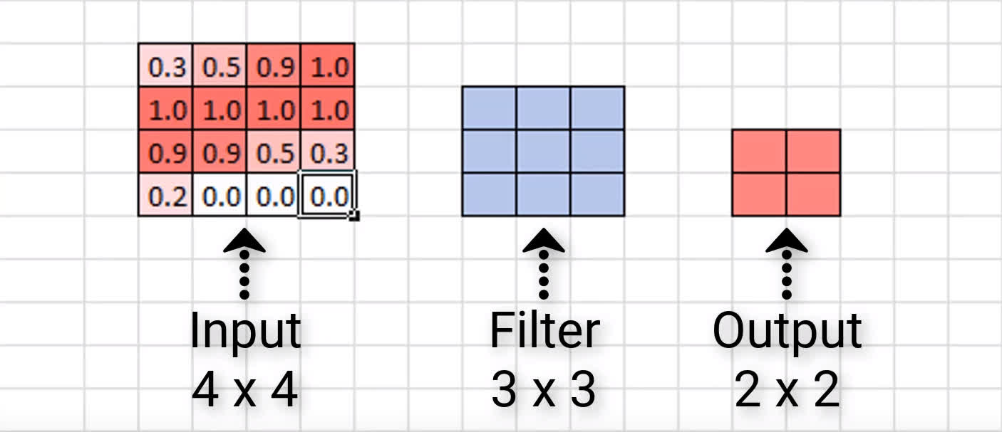
Let’s see if this holds up with our example here.
Indeed, this gives us a 2 x 2 output channel, which is exactly what we saw a moment ago. This holds up for the example with the larger input of the seven as well, so check that for yourself to confirm that the formula does indeed give us the same result of an output of size 26 x 26 that we saw when we visually inspected it.
Issues with reducing the dimensions
Consider the resulting output of the image of a seven again. It doesn’t really appear to be a big deal that this output is a little smaller than the input, right?
We didn’t lose that much data or anything because most of the important pieces of this input are kind of situated in the middle. But we can imagine that this would be a bigger deal if we did have meaningful data around the edges of the image.
Additionally, we only convolved this image with one filter. What happens as this original input passes through the network and gets convolved by more filters as it moves deeper and deeper?
Well, what’s going to happen is that the resulting output is going to continue to become smaller and smaller. This is a problem.
If we start out with a 4 x 4 image, for example, then just after a convolutional layer or two, the resulting output may become almost meaningless with how small it becomes. Another issue is that we’re losing valuable data by completely throwing away the information around the edges of the input.
What can we do here? Queue the super hero music because this is where zero padding comes into play.
Zero padding to the rescue
Zero padding is a technique that allows us to preserve the original input size. This is something that we specify on a per-convolutional layer basis. With each convolutional layer, just as we define how many filters to have and the size of the filters, we can also specify whether or not to use padding.
What is zero padding?
We now know what issues zero padding combats against, but what actually is it?
Zero padding occurs when we add a border of pixels all with value zero around the edges of the input images. This adds kind of a padding of zeros around the outside of the image, hence the name zero padding. Going back to our small example from earlier, if we pad our input with a border of zero valued pixels, let’s see what the resulting output size will be after convolving our input.
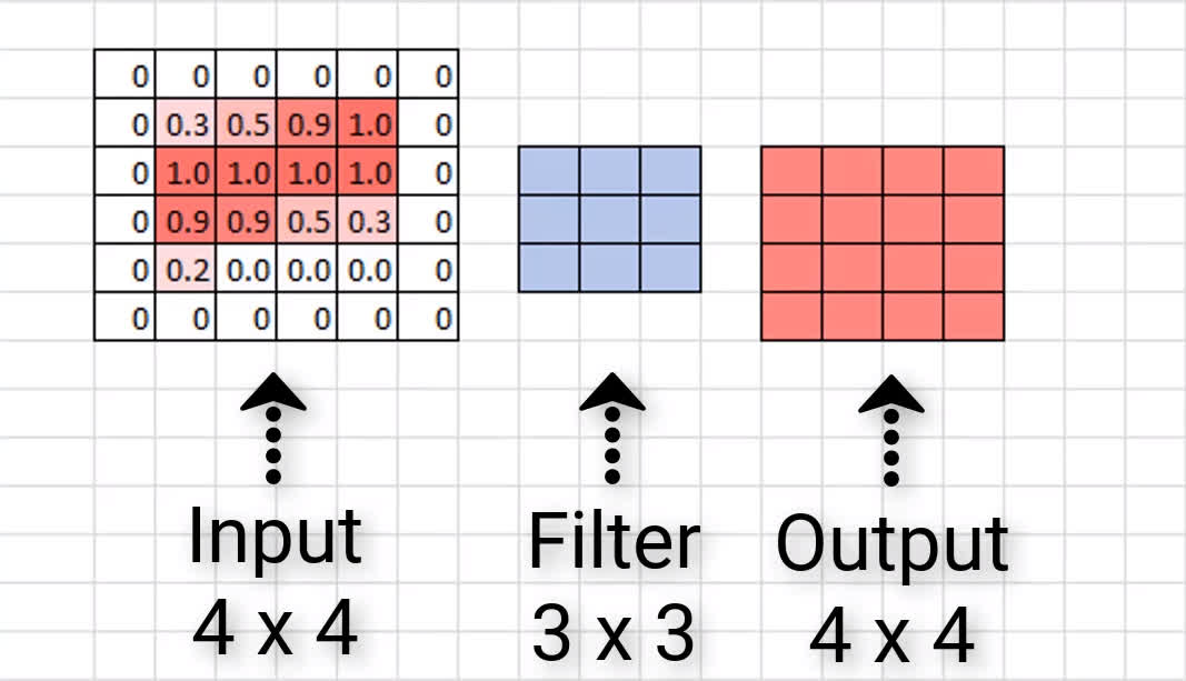
The good thing is that most neural network APIs figure the size of the border out for us. All we have to do is just specify whether or not we actually want to use padding in our convolutional layers.
Valid and same padding
There are two categories of padding. One is referred to by the name valid. This just means no padding. If we specify valid padding, that means our convolutional layer is not going to pad at all, and our input size won’t be maintained.
The other type of padding is called same. This means that we want to pad the original input before we convolve it so that the output size is the same size as the input size.
| Padding Type | Description | Impact |
|---|---|---|
| Valid | No padding | Dimensions reduce |
| Same | Zeros around the edges | Dimensions stay the same |
Now, let’s jump over to Keras and see how this is done in code.
Working with code in Keras
Now, we’ll create a completely arbitrary CNN.
It has a dense layer, then 3 convolutional layers followed by a dense output layer.
This is actually the default for convolutional layers in Keras, so if we don’t specify this parameter, it’s going to default to valid padding. Since we’re using valid padding here, we expect the dimension of our output from each of these convolutional layers to decrease.
Let’s check. Here is the summary of this model.
So, we start with 20 x 20 and end up with 8 x 8 when it’s all done and over with.
On the contrary, now, we can create a second model.
This one is an exact replica of the first, except that we’ve specified same padding for each of the convolutional layers. Recall from earlier that same padding means we want to pad the original input before we convolve it so that the output size is the same size as the input size.
Let’s look at the summary of this model.
This is why we call this type of padding same padding. Same padding keeps the input dimensions the same.